An Introduction to Elastic Stability and pyfurc – A Tutorial

This tutorial first explains some mechanical and mathematical background and thereafter demonstrates the basic usage of pyfurc by solving one of the simplest example problems in elastic stability.

Problem: The Hinged Cantilever

Consider the rigid cantilever with length \(\ell\) shown below. On the top end it is subject to a dead load \(P\). On the bottom end there is a simple support as well as a torsional spring with stiffness \(c_T\).

Fig. 1: Hinged Cantilever

The angle \(\varphi\) measures the rotation of the cantilever with respect to the vertical axis.

Our first aim is to find a relationship between the load \(P\) and the cantilever rotation \(\varphi\).

1. The Introductory Mechanics Approach

The moment equilibrium taken in the deflected position (shown right in the figure above) dictates that

\[P\ell\sin\varphi-c_\mathrm{T}\varphi=0\,.\]

We now have the task to find all valid tuples \((P,\varphi)\) which satisfy the above equation. We constrain ourselves to the sensible choice \(0\leq|\varphi|\leq\frac\pi2\).

Apparently, for \(\varphi=0\) we can choose an arbitrary value for \(P\) and the equilibrium condition is satisfied. This corresponds to the trivial, non-deflected solution and we will later see that this equilibrium state is only stable up to a certain point.

For \(\varphi\neq0\) let us set \(\bar P=\frac {P\ell}{c_\mathrm{T}}\) such that the relation becomes

\[\bar P = \frac\varphi{\sin\varphi}\,.\]

With this expression we have fulfilled our task of finding tuples that satisfy the equilibrium condition. These solutions are also called equilibrium paths and are plotted below:

Fig. 2: Equilibrium paths of the hinged cantilever system: The red curve corresponds to the non-trivial solutions, the black curve to the trivial solution.

As we can see, for \(\bar P>1\) we have multiple possible solutions for \(\varphi\). Graphically we can identify \(\bar P=1\) as a critical point or bifurcation point. When continually loading the system from zero load, the path it takes after reaching \(\bar P=1\) is non-unique. Both paths are mechanically equally valid and admissible as they both satisfy the equilibrium condition. In reality, small imperfections, e.g. deviations in the angle of the applied load, bearing friction, a not perfectly straight cantilever etc. will always nudge the system into taking a preferred equilibrium path.

Systems like this, which do not have a unique solution for a given input are not easily tackled computationally. Standard algorithms may find only one of many solution paths or never converge to a solution at all. Of course in this simple problem we were able to find the solutions analytically but this surely is not the case for most systems.

This is where the FORTRAN program AUTO-07p comes into play in which sophisticated algorithms that can handle non-uniqueness, bifurcations and unstable solutions are implemented and allow for numerical solutions of such systems with bifurcations.

Pyfurc facilitates this functionality. But before diving in, let us introduce a more systematic approach to elastic systems than taking the Newton equilibrium equations.

2. The Total Potential Energy Method

This section will give a brief introduction to the total potential energy (TPE) method which provides a way to systematically tackle a broad class of elastic systems. For more a more in-depth introduction we recommend the book by Thompson & Hunt (1973)[1].

The total potential energy \(V\) of an elastic system is given by an internal potential energy \(U\) minus the work done by external forces. We restrict ourselves to systems which are subject to only one load \(P\). This load does work along a path \(\Delta\). The internal energy as well as the path \(\Delta\) may be functions of the degrees of freedom \(Q_i\) of the system.

Thus the TPE takes the following general form:

\[V(Q_i, P)=U(Q_i)-P\Delta(Q_i)\,.\]

Note

Before you continue…

What is the only degree of freedom in our example system?

Try figuring out the TPE of the hinged cantilever.

The TPE method relies on the following two axioms:

• Axiom 1:

  A stationary value of the total potential energy with respect to the generalized coordinates is necessary and sufficient for the equilibrium of the system.

• Axiom 2:

  A complete relative minimum of the total potential energy with respect to the generalized coordinates is necessary and sufficient for the stability of an equilibrium state.

Equilibrium

Mathematically the first axiom translates to

\[\frac{\partial V}{\partial Q_i} = 0 \quad\Leftrightarrow\quad \textrm{Equilibrium}.\]

Thus, to find equilibrium states of a system we need to

1. identify/define the degrees of freedom,

2. formulate the TPE expression

3. and take its first derivatives w.r.t. all degrees of freedom.

The result is a set of equations (as many as there are degrees of freedom), the solutions of which correspond to all equilibrium states of the system.

Let us perform these three steps for our example system from above:

1. The system has only one degree of freedom, the bottom support restricts translatory movement in horizontal and vertical direction but allows for rotational movement. The sensible choice is setting \(Q_1=\varphi\).

2. We neglect gravitational potential energy and find that the only potential energy in the system is inside the torsional spring, thus:

   \[U(\varphi) = \frac12c_\mathrm{T}\varphi^2\]

   The force \(P\) does work along the displacement

   \[\Delta(\varphi) = \ell(1-\cos\varphi)\]

   Combining these results gives the TPE

   \[V(\varphi, P) = \frac12c_\mathrm{T}\varphi^2-P\ell(1-\cos\varphi)\]

3. Taking the derivative w.r.t to all degrees of freedom, i.e. \(\varphi\), and applying the first axiom yields:

   \[\frac{\partial V}{\partial\varphi} = c_\mathrm{T}\varphi - P\ell\sin\varphi=0\]

The above result is exactly the same equilibrium equation we found by using Newton’s equation of motion. But we got there through a more systematic approach which translates well to more complicated systems with more degrees of freedom.

Stability

The second axiom states that for an equilibrium state to be stable it has to be a local minimum. Mathematically we can assert this by taking a Taylor series expansion about an equilibrium state.

Let us suppose we have found an equilibrium state \(\bar Q\) of a system with one degree of freedom \(Q\) using the above method. The change in energy when altering the equilibrium state \(\bar Q\) by a small amount \(\varepsilon\) then reads

\[V(\bar Q+\varepsilon)-V(\bar Q)= \frac1{2!}\frac{\partial^2 V}{\partial Q^2}\bigg|_{Q=\bar Q}\varepsilon^2 + \frac1{3!}\frac{\partial^3 V}{\partial Q^3}\bigg|_{Q=\bar Q}\varepsilon^3 + \frac1{4!}\frac{\partial^4 V}{\partial Q^4}\bigg|_{Q=\bar Q}\varepsilon^4+\ldots\]

Note that the first derivative is missing in the expression above since for an equilibrium state it has to vanish according to axiom 1. We are also omitting the load parameter \(P\) for brevity.

Now for \(V(\bar Q)\) to be a minimum, i.e. for \(\bar Q\) to be a stable equilibrium state after axiom 2, the above change in energy has to be positive for any \(\varepsilon\). This means that the first nonzero term in the series expansion must be positive for any \(\varepsilon\). It thus has to be a term with an even power of \(\varepsilon\) and a positive corresponding coefficient.

If the whole series is zero the equilibrium is called neutrally stable. Any other case is called an unstable equilibrium.

If only

\[\frac{\partial^2 V}{\partial Q^2}\bigg|_{Q=\bar Q}=0\]

in an equilibrium state \(\bar Q\) then the energy function is locally flat. This implies a change in the system’s stability and is called singular, critical or bifurcation point.

Now let us check the stability for the equilibrium states of our example system. To this end, we start by analyzing the first even order derivative:

\[\frac{\partial^2 V}{\partial \varphi^2} = 1-\bar P\cos(\varphi)\]

Obviously, for \(\bar P<1\) this expression is positive for arbitrary values of \(\varphi\). Thus, our trivial equilibrium path where \(\varphi=0\), is stable up to \(\bar P = 1\) where the second derivative becomes zero. For \(\bar P > 1\) the second derivative is negative and thus, the trivial equilibrium states are unstable for \(\bar P>1\). We marked these unstable states with a dashed line in the diagram in Fig. 2 whereas solid lines show the stable equlibrium states.

Now for the non-trivial equilibrium solutions

\[\bar P =\frac{\varphi}{\sin\varphi}\,.\]

Plugging these into the expression for the second derivative gives

\[\frac{\partial^2 V}{\partial Q^2}\bigg|_\mathrm{eq.}=1-\frac{\varphi}{\tan\varphi}\]

which is always positive for our chosen interval of \(0\leq|\varphi|\leq\frac\pi2\). All these equilibrium states are thus stable.

Take a look at the figure below where the TPE function \(V(\varphi, \bar P)\) is plotted over the normalized angle \(\frac{2\varphi}\pi\) and the normalized load \(\bar P = \frac{P\ell}{c_\mathrm{T}}\). It should be clear why \(V\) is sometimes called energy surface or energy landscape

On this energy surface, the equilibrium states we found earlier are plotted. The figure is interactive! Hovering over the energy surface will show you the function \(V(\varphi)\) for a fixed value of \(\bar P\) as a dark blue line across the energy surface. On these curves you can clearly see the local minima the stable equilibrium paths pass through as well as the local maxima the unstable path passes through. You can also observe the locally flat surface at the critical point \(\bar P = 1\).

Take a little time to play around with the visualization, rotate the graph, zoom in and out to identify the observations stated above.

Note that we did not provide a numeric scale for the values of the energy function. This is because the absolute value of the TPE has no influence on the mechanical behaviour of the system. Recall that it is only the derivatives that are relevant for the mechanical response, i.e. equilibrium and stability.

Also note that a visualisation like this is only possible for systems with exactly one degree of freedom subject to exactly one load. Only then a surface can be plotted as a function of the degree of freedom and the load parameter.

3. Numerical Solution with pyfurc

Let us recap what we had to do to find the equilibrium states of our example system using the TPE method:

1. Identify/define the degrees of freedom,

2. formulate the TPE expression

3. and take its first derivatives w.r.t. all degrees of freedom to obtain the equilibrium equations.

4. Find all states that satisfy the equilibrium equations.

Pyfurc takes over after step 2. Based on a provided expression for the TPE pyfurc determines the equilbrium equations and solves them via AUTO-07p.

For this example system we could obtain the solutions analytically and finding the equilibrium equations was a trivial task. But for more complicated systems, obtaining analytical solutions may be impossible and determining the equilibrium equations may become tedious.

Note

If you already have installed pyfurc you can just follow along and try everything out yourself, preferrably in a jupyter notebook. Otherwise go to this page for installation instructions.

We have already gone through steps 1 and 2 above: Our only degree of freedom is \(\varphi\) and our TPE reads

\[V(\varphi, P) = \frac12 c_\mathrm{T}\varphi^2-P\ell(1-\cos\varphi)\,.\]

The first thing we do is import pyfurc and sympy. The latter is a symbolic math package for python and enables us to define the TPE as a symbolic expression.

import pyfurc as pf
import sympy as sp

We can now define the degree of freedom \(\varphi\) as pf.Dof, the load \(P\) as pf.Load as well as the constants \(c_T\) and \(\ell\) as simple floating point numbers.

phi = pf.Dof("\\varphi")
P = pf.Load("P")
c_T = 1
ell = 1

The only argument we have to supply inside the brackets is the name the variable has for display purposes. Since the backslash is reserved as a special character in python strings we have to escape it using another backslash. The strings we supplied can be rendered using LaTeX, which is why we called our dof \\varphi.

If you are inside a jupyter notebook you can run display(phi) and it should output a rendered phi.

With the above quantities defined we can define the energy expression using

V = pf.Energy(1/2*c_T*phi**2 - P*ell*(1-sp.cos(phi)))

Note that we use the cos function supplied by sympy which we imported above as sp. The only argument for pf.Energy is the expression.

Recall that when solving the problem manually we would now determine the equilibrium equations by calculating the first derivatives. In pyfurc we instead define a pf.BifurcationProblem as follows:

bf = pf.BifurcationProblem(V, name="hinged_cantilever")

The first (mandatory) argument here is the energy expression V. The second argument is an optional keyword argument that is used to name output files.

The pf.BifurcationProblem object holds parameters and settings for the calculation. One important parameter is called RL1 (by AUTO-07p) which is the maximum load up to which the calculation is carried out. For our choice of constants, setting this to 2.0 is sensible (can you give a reason why this is the case?):

bf.set_parameter("RL1", 2.0)

The rest of the parameters inside the pf.BifurcationProblem is kept at default values which can be found here.

The last step is to define and run the solver:

solver = pf.BifurcationProblemSolver(bf)
solver.solve()

If solver.solve() has run successfully, you will get a console output by AUTO-07p which has been called in the background. More importantly, our BifurcationProblem now holds the solutions as a list of pandas DataFrames inside bf.solution.raw_data. Each list item corresponds to a single equilibrium branch.

We can create a very rudimentary plot with the following lines:

import matplotlib.pyplot as plt
for branch in bf.solution.raw_data:
    plt.plot(branch["U(1)"], branch["PAR(1)"])

In the lines above we iterate over the DataFrames in bf.solution.raw_data and plot their respective U(1) (i.e. the first DOF in AUTO-07p nomenclature) and PAR(1) (i.e. the first load parameter in AUTO-07p nomenclature) columns using matplotlib. The resulting plot should look more or less like this:

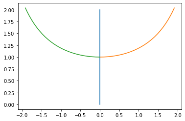
Fig. 3: Rudimentary Bifurcation Plot

If you prefer to work with the actual raw data output by AUTO-07p, a directory with the name of the BifurcationProblem and a timestamp should have been created inside the directory where you have run your python script. In this case, the directory is called hinged_cantilever_YYYYMMDD_HHMMSS and you can find the generated FORTRAN code hinged_cantilever.f90 and its compiled executable, the output files fort.7, fort.8 and fort.9 as well as the constants file c.hinged_cantilever inside.

The complete code for the above example looks as follows:

import pyfurc as pf
import sympy as sp
import matplotlib.pyplot as plt

phi = pf.Dof("\\varphi")
P = pf.Load("P")
c_T = 1
ell = 1

V = pf.Energy(1/2*c_T*phi**2 - P*ell*(1-sp.cos(phi)))
bf = pf.BifurcationProblem(V, name="hinged_cantilever")
bf.set_parameter("RL1", 2.0)

solver = pf.BifurcationProblemSolver(bf)
solver.solve()

for branch in bf.solution.raw_data:
    plt.plot(branch["U(1)"], branch["PAR(1)"])

Congratulations! You have successfully solved your first bifurcation problem with pyfurc!

Literature

[1]

J.M.T. Thompson and G.W. Hunt. A General Theory of Elastic Stability. Wiley-Interscience publication. J. Wiley, 1973.